School of Population Health

Appendix 3. Partition criteria

Referring to the Criteria dialog, there are 8 options for assessing partitions:

A3.1 Within MSE

This is the measure described in reference 2 equation (7), viz.,

where i is impurity measured by mean-square-error, for example, in A,

where i(A∪A- ) refers to impurity of the whole sample. This measure can be calculated for interval, nominal or binary Y. However, note that for nominal Y, the coded numbers of the categories are treated simply as their numeric coded value, so that the index may not have a sensible interpretation.

For binary Y, G is the same as the Gini index of diversity (see below), apart for a factor 2.

A3.2 Subgroup MSE

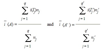
This is the measure described in Reference 2 measuring the effectiveness a partition in terms of its constituent subgroups. Specifically:

where

and where impurity i is mean square error.

This measure can be used for any Y, as for the Within MSE measure. Note that it is possible for negative values of G to arise with this index.

My experience with it now is that it is best avoided. It may give subgroups that are reasonably pure with respect to the outcome, but, apparently paradoxically, not necessarily good overall purity in terms of A and A-.

A3.3 Entropy

This is as in equation (1) but with an entropy measure instead of mean square error measuring impurity. It is allowed for nominal outcomes, with up to 10 categories (represented by digits 0,1, to 9).

Suppose there are k categories and p = p₁,...,p_k are probabilities assigned to each. Then i() is defined as

The entropy measure is then

where $\pi \!\,$ is the distribution in the whole sample, p_A in A and p_A- in A-. Note that the entropy measure does not extend to equation (2), that is, you cannot use a subgroup purity measure with other than mean square error for impurity.

A3.3.1 Prior probabilities

In general the $\pi \!\,$ 's in the above are the sample proportions in the data. However, you can specify the $\pi \!\,$ 's accounting for prior probabilities. Suppose $\pi \!\,$ ₁,..., $\pi \!\,$ _k are specified prior probabilities for each category of the outcome. Then you can work out the first term i( $\pi \!\,$ ) in (3) with these values. 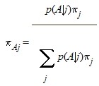The $\pi \!\,$ _A and $\pi \!\,$ _A- are then calculated from the data and the $\pi \!\,$ _j's. Specifically, using Bayes formula the jth element of $\pi \!\,$ _A is

where p(A|j) is the proportion of the data in category j with A.

There are three radio buttons to assign priors in the Criteria dialog box: Data priors are the sample proportions in the whole data; Equal priors assign $\pi \!\,$ _j = 1/k; User priors are values input by the user.

A3.4 Quality index QI(r)

This is the quality index QI(r) of a 2 by 2 table as described by Kraemer (reference 4, equation 6.1). Only applicable for binary Y. The relative cost r is set by the Costs that are assigned, so the Specify Costs button must be checked in the Criteria dialog. The r value is calculated by the proportion of excess costs. For example, for the following specified costs the excess cost for outcome 1 is (5-1)=4 and for outcome 0 it is (10-2)=8, so that r=4 / (8+4)=0.33

The program will automatically invoke a "turbo" facility to speed the computations ifOption:Turbo on is checked. This is done by pre-processing and collapsing the data into identical groups of observations according to the number of distinct values of Y, say n_Y, and the m binary elements of the attribute set. The process is only invoked if n_Y < 10 and m + n_Y - 1 ≤ 15, otherwise the storage requirements become heavy to implement the collapse and the benefits are minimal.

However, the computational gains can be enormous when the data set is large. For example, one test data set with about 50,000 observations and binary Y collapsed to just 279 distinct groups, of the 2¹⁵ = 32768 possible combinations with m + n_Y - 1 = 15. The effective number of records was therefore 279 rather than 50,000.

Searches with large sample sample sizes (e.g 50,000) can be slow, for any Y that has more than a few distinct values. The procedure may also not be invoked when the cuts of an attribute are allowed to float (see 14.4). Each possible cut is considered to be included in defining m. So that, for instance, in creating a tree where you would normally float cuts, the turbo facility may not be invoked.

If you have a very large data set for which records are not unique, it is a good idea to pre-process the data by collapsing it into grouped form and using the _freq_ input count variable.

Another factor that affects the time for a search is the complexity of Boolean expressions that define the partition. The additional time required for complex partitions may arise in the manipulation of Boolean expressions. If an iterative search is done that does not converge and continues to generate more and more complex partitions, performance will slow. In this case try increasing the complexity penalising parameter.

A3.5 Chi-square

This is the usual chi-square statistic, not corrected for continuity. It can only be used for a Ythat is defined as nominal, ordinal or binary in the control file. Accordingly, the categories of Ymust be coded with a single digit and limited to 10 possible values (see 9.3.1)

Note that for a 2 by 2 table, chi-square is the well known quantity

where A,B,C,D are marginal totals with A,B sums in A and A- and C and D the sums in the two groups of Y. If you use this measure and the balancing option with ɣ = 1 the statistic is

since C and D are fixed. In other words, the measure is equivalent to |ad-bc| which has sometimes been suggested as an effectiveness measure.

Note also that as χ²/^N = ϕ², where f is the so- called phi-coefficient, using χ² is equivalent to using ϕ², which is itself the same thing as the multiple correlation coefficient and is a good prognostic discriminator for binary outcomes (see Buyse, M. Statistics in Medicine, 18, 271-274 (2000)).

A3.6 Odds ratio (Bayes)

This is only applicable to binary Y and is the quantity

where a,b,c,d are counts in the 4 cells. This is a Bayes estimator in the sense that augmenting each cell by unity is equivalent to prior information of one observation in each cell.

A3.7 Log-rank statistic

This is the log-rank statistic for testing differences between two survival functions. The outcome measure may be censored. If it is, you must have an attribute that signifies censoring. You will be shown a menu of all created attributes and asked to pick the one that indicates censoring. None of the other effectiveness measures allow for censoring. SPAN takes no account of possible tied values in the computation of log-rank.

When log-rank is selected SPAN enters a mode in which incidence rates and incidence rate ratios are output rather than means.

You cannot have a multivariate log-rank measure.

A3.8 Gini diversity

This is as in equation (1) but with a Gini index of diversity measure instead of mean square error measuring impurity. It is allowed for nominal outcomes, with up to 10 categories (represented by digits 0 to 9).

Suppose there are k categories and p_j; j = 1,...,k are probabilities assigned to each. Then i() is defined as

Note that this measure does not extend to equation (2), that is, you cannot use a subgroup purity measure with other than mean square error for impurity.

The index can be specified with user defined prior probabilities, as for the Entropy index (see A3.3.1).

Suppose there are k categories and p_j; j = 1,...,k are probabilities assigned to each. Then i() is defined as

Note that this measure does not extend to equation (2), that is, you cannot use a subgroup purity measure with other than mean square error for impurity.

The index can be specified with user defined prior probabilities, as for the Entropy index (see A3.3.1).

A3.9 Directional v. Non-directional indices

Note that, with the exception of the Odds ratio and Quality indices, all the effectiveness criteria are non-directional, in the sense that, for example, a partition A = { x = 0}, for a binary variable x, will score precisely the same as A = { x = 1}. That is, non- directional effectiveness measures do not explicitly assess the SPAN paradigm: "A corresponds to high Yand A- to low Y" (see 3). However, provided positive attributes are appropriately constructed, so that they are indicative of high Y, the situation where the best partition is the reverse of the SPAN paradigm is unlikely to occur, unless the synergistic effect of a combination of positive attributes produces a complete reversal of the individual effects.

Note, however, that when ranking univariate partitions (see 12) with a non-directional measure, partitions that are the reverse of the SPAN paradigm may score well. For example, in the extreme situation in which two attributes {x = 0} and {x = 1} are created and each assigned a positive designator (which can be achieved by having consecutive lines x b 1 and x b 0 in the control file), both attributes will be tied on the ranking procedure.

A3.10 Multiple Y measures

When a multivariate set of outcomes is selected, say Y = (Y₁,Y₂,..., Y_k) the multiple effectiveness measure is the sum of the individual measures of the Y_r's. For example, if G_r is the measure for Y_r the multiple measure is

If the individual Yr are measured on quite different scales it is sometimes sensible to re-scale the Yr by dividing each by the overall sample variance. This is equivalent to attaching a weight to the sum in (4), that is, forming

where w_r = 1/s_r² is the inverse sample variance of Y_r. When multiple Y is selected you can tick the inverse variance weighting in the Criteria dialog box.

When G_r in (4) is the within MSE in (1), it can be shown that maximising (4) is equivalent to maximising the Euclidean distance metric

where

is the total distance in the k-dimensional space between observations, and DA and DA- are corresponding measures in A and A-. In other words, using multiple Y can be considered as a means to form two "clusters" in k- dimensional space, A and A-, that are homogeneous with respect to Y. The clusters are defined by attributes rather than in a conventional cluster analysis where they are specified only by their observation number.

There are certain restrictions on specifying multivariate Y: you cannot use the Gini or Entropy measures with user specified probabilities and you cannot use the log-rank criterion.

[Back to table of contents]

SPAN

SCHOOLS, DEPARTMENTS AND CENTRES